Modevectors: Difference between revisions
No edit summary |
PedroLacerda (talk | contribs) No edit summary |
||
| (53 intermediate revisions by 5 users not shown) | |||
| Line 1: | Line 1: | ||
{{Infobox script-repo | |||
|type = script | |||
|filename = scripts/modevectors.py | |||
|author = [[User:Slaw|Sean M. Law]] | |||
|license = - | |||
}} | |||
===DESCRIPTION=== | ===DESCRIPTION=== | ||
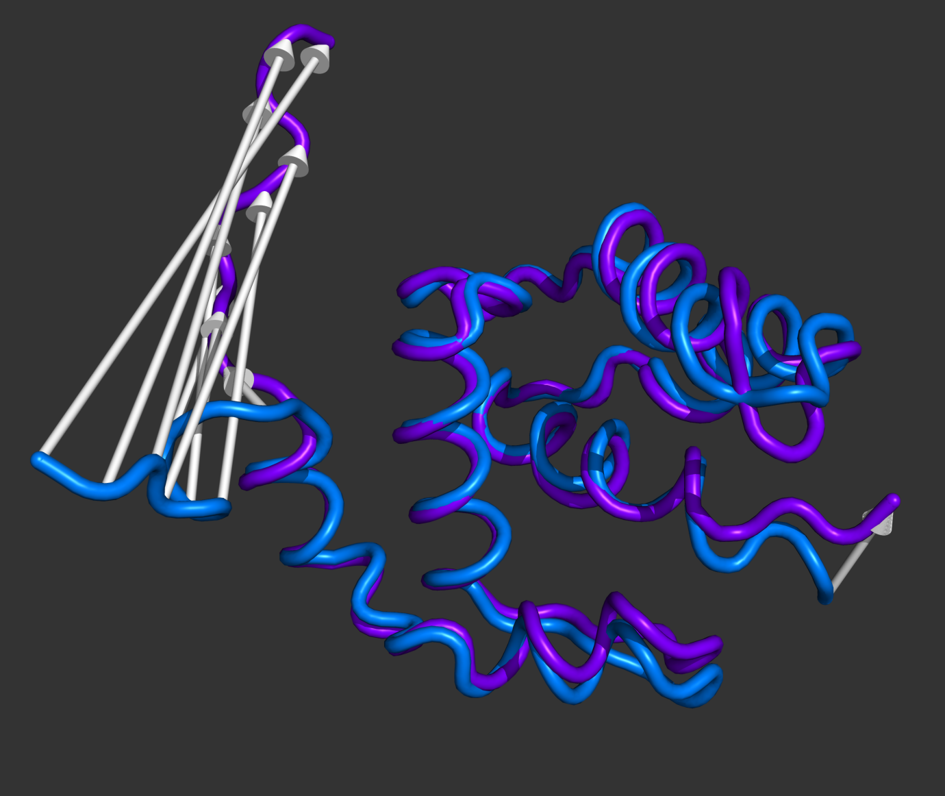
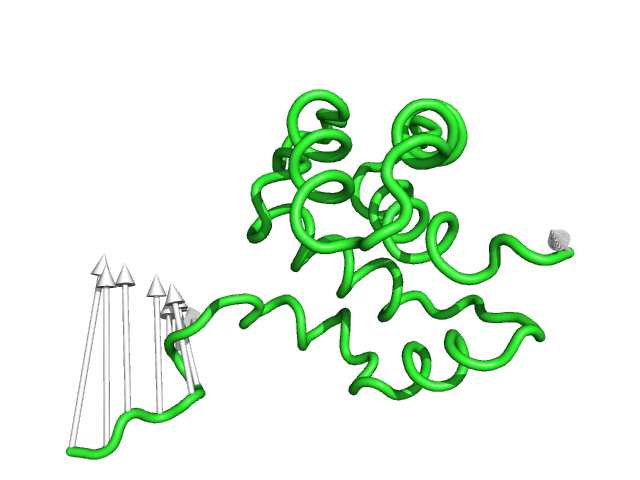
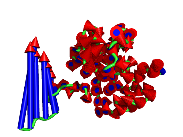
'''modevectors.py''' is a PyMol script that was originally written to visualize results obtained from Normal Mode Analysis (NMA). However, this script can be used to visualize the direction of motion between two specified states. The strength of this script is that the arrows are highly customizable with numerous options to choose from (see script below). | [[Image:Modevectors.png|right|thumb|250px|Example showing modevectors in action. (See Examples below).]] | ||
'''modevectors.py''' is a PyMol script that was originally written to visualize results obtained from Normal Mode Analysis (NMA) by drawing arrows or vectors from a starting structure to a final structure. However, this script can be used to visualize the direction of motion between two specified states (e.g. targeted MD, comparing open and closed structures, etc). The strength of this script is that the arrows are highly customizable with numerous options to choose from (see script below). It is important to note that the two states MUST be identical except for the X, Y, and Z coordinates. That is, you cannot draw vectors between homologous structures. The default settings sets the background to white and displays the arrows along with the first object frame (in cartoon representation). | |||
Note: Ray tracing these CGO arrows appears to be a memory intensive process so please save a session before ray tracing and use "pymol -qc" where necessary. If anybody can come up with a method to improve this please e-mail me (see address in script). | |||
Update: A new way of drawing the arrows has been implemented for PyMOL v.1.1 and has been updated in this code (which automatically detects the version that you are using). The new method uses the built in cone primitive rather than concentric circles decreasing in size. Thus, the new method is much less memory intensive and is a significant improvement over the old method. Additionally, you may want to turn off [[ray shadow]] depending on the [[scene]] that you are viewing as shadows can be confusing to others when seen in publications. | |||
===USAGE=== | ===USAGE=== | ||
| Line 7: | Line 21: | ||
<source lang="python"> | <source lang="python"> | ||
modevectors first_obj_frame, last_obj_frame [,outname=modevectors [,head=1.0 [,tail=0.3 [,head_length=1.5 [,headrgb=(1.0,1.0,1.0) [,tailrgb=(1.0,1.0,1.0) [,cutoff=4.0 [,skip=0 [,cut=0.5 [,atom=CA [,stat=show [,factor=1.0]]]]]]]]]]] | modevectors first_obj_frame, last_obj_frame [,first_state=1 [,last_state=1 [,outname=modevectors \ | ||
[,head=1.0 [,tail=0.3 \[,head_length=1.5 [,headrgb=(1.0,1.0,1.0) [,tailrgb=(1.0,1.0,1.0) [,cutoff=4.0 | |||
[,skip=0 [,cut=0.5 [,atom=CA [,stat=show [,factor=1.0 [,notail=0]]]]]]]]]]]]]] | |||
</source> | </source> | ||
| Line 20: | Line 36: | ||
</source> | </source> | ||
Copy/paste the following code to see an example of modevectors. This uses a multistate protein and the arrows are connected between the first and last states. | |||
<source lang="python"> | |||
import modevectors | |||
# fetch the PDBs from pdb.org | |||
fetch 1c3y, finish=1, multiplex=0, async=0 | |||
# separate the first and last states of the NMR ensemble to individual objects | |||
split_states 1c3y, 1, 1 | |||
split_states 1c3y, 23, 23 | |||
hide | |||
# run the modevectors code | |||
modevectors 1c3y_0001, 1c3y_0023 | |||
# just setup a nice representation | |||
as cartoon, 1c3y_0001 or 1c3y_0023 | |||
show cgo, modevectors | |||
color marine, 1c3y_0001 | |||
color purpleblue, 1c3y_0023 | |||
</source> | |||
The following set of examples will illustrate the power of each optional argument. Each example should be compared to the default figure in the table below. | |||
{| | |||
|[[Image:mv_default.png|thumb|300px|left|Fig.1 - Default Settings]] | |||
||[[Image:mv_fig2.png|thumb|300px|left|Fig.2 - Arrow direction drawn from CA to CA]] | |||
||[[Image:mv_fig3.png|thumb|300px|left|Fig.3 - Arrow head radius]] | |||
|- | |||
|[[Image:mv_fig4.png|thumb|300px|left|Fig.4 - Arrow tail radius]] | |||
||[[Image:mv_fig5.png|thumb|300px|left|Fig.5 - Arrow head length]] | |||
||[[Image:mv_fig6.png|thumb|300px|left|Fig.6 - Arrow head RGB]] | |||
|- | |||
|[[Image:mv_fig7.png|thumb|300px|left|Fig.7 - Arrow tail RGB]] | |||
||[[Image:mv_fig8.png|thumb|300px|left|Fig.8 - Arrow length cutoff]] | |||
||[[Image:mv_fig9.png|thumb|300px|left|Fig.9 - Skip every other arrow]] | |||
|- | |||
|[[Image:mv_fig10.png|thumb|300px|left|Fig.10 - Subtract value from vector length]] | |||
||[[Image:mv_fig11.png|thumb|300px|left|Fig.11 - Draw arrows from CB atoms]] | |||
||[[Image:mv_fig12.png|thumb|300px|left|Fig.12 - Shorten by 50%]] | |||
|- | |||
|||[[Image:mv_fig13.png|thumb|300px|left|Fig.13 - Multiple options being used (see final example below)]] | |||
|} | |||
<syntaxhighlight lang="python"> | |||
reinitialize | |||
import modevectors | |||
fetch 1c3y, async=0 | |||
split_states 1c3y, 1, 1 | |||
split_states 1c3y, 23, 23 | |||
hide | |||
#This is the default setting (Fig.1) | |||
modevectors 1c3y_0001, 1c3y_0023 | |||
#This is shows that the direction of the arrows is drawn from the 1c3y_0001 towards 1c3y_0023 (Fig.2) | |||
show cartoon, 1c3y_0023 | |||
color red, 1c3y_0023 | |||
#This controls the base radius of the cone/arrow head in angstroms (Fig.3) | |||
modevectors 1c3y_0001, 1c3y_0023, head=2.5 | |||
#This controls the radius of the cylinders/arrow tails in angstroms (Fig.4) | |||
modevectors 1c3y_0001, 1c3y_0023, tail=0.75 | |||
#This controls the length of the cone/arrow head in angstroms (Fig.5) | |||
#Note that this option does NOT increase the vector length but simply changes the tail length | |||
modevectors 1c3y_0001, 1c3y_0023, head_length=3.0 | |||
#This controls the colour of the cone/arrow head using RGB values (Fig.6) | |||
modevectors 1c3y_0001, 1c3y_0023, headrgb=(1.0,0.0,0.0) | |||
#This controls the colour of the cylinder/arrow tails using RGB values (Fig.7) | |||
modevectors 1c3y_0001, 1c3y_0023, tailrgb=(1.0,0.0,0.0) | |||
#This controls the which vectors to show based on a specific cutoff value in angstroms. Vector lengths that are less | |||
#than the cutoff value will not be displayed (Fig.8) | |||
modevectors 1c3y_0001, 1c3y_0023, cutoff=30.0 | |||
#This controls how many vectors to skip (integer value) and is useful when there are too many vectors showing. | |||
#Skip=1 will show every other arrow (Fig.9) | |||
modevectors 1c3y_0001, 1c3y_0023, skip=1 | |||
#This controls how much to cut from each vector (in angstroms). Note that arrows will point in the opposite directions | |||
#when too much is cutoff (resulting in a negative vector length) (Fig.10) and should be used with caution! | |||
modevectors 1c3y_0001, 1c3y_0023, cut=15.0 | |||
#This controls which atom to draw a vector from (Fig.11). Note that this is case-sensitive and is really only useful | |||
#when atom=CA or when atom=P (for DNA backbones) | |||
modevectors 1c3y_0001, 1c3y_0023, atom=CB | |||
#This controls how much to multiple the length of each vector by (percentage increase/decrease) (Fig.12) | |||
#This example halves the length of each vector (50%) | |||
modevectors 1c3y_0001, 1c3y_0023, factor=0.5 | |||
#This hides the statistics which count atoms skipped, atoms counted (number of arrows showing), and number of atoms | |||
#that did not meet the cutoff and are not shown | |||
modevectors 1c3y_0001, 1c3y_0023, stat=hide | |||
#This example shows multiple options being used (Fig.13) | |||
modevectors 1c3y_0001, 1c3y_0023, head=2.0, tail=1.0, head_length=2.0, headrgb=(1.0,0.0,0.0), tailrgb=(0.0,0.0,1.0), | |||
cutoff=0.0,skip=0,cut=0,atom=CA,factor=0.8 | |||
#Finally, this example hides all arrow tails and only uses arrow heads via the notail option(No Figure) | |||
modevectors 1c3y_0001, 1c3y_0023, head=2.0, cutoff=0.0,skip=0,cut=0,atom=CA,factor=0.8, notail=1 | |||
</syntaxhighlight> | |||
[[Category:Script_Library]] | |||
[[Category:Math_Scripts]] | |||
[[Category:Pymol-script-repo]] | |||
Latest revision as of 21:45, 22 June 2025
| Type | Python Script |
|---|---|
| Download | scripts/modevectors.py |
| Author(s) | Sean M. Law |
| License | - |
| This code has been put under version control in the project Pymol-script-repo | |
DESCRIPTION
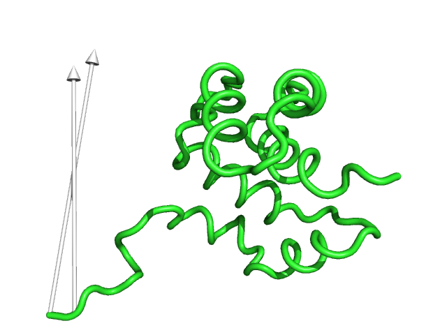
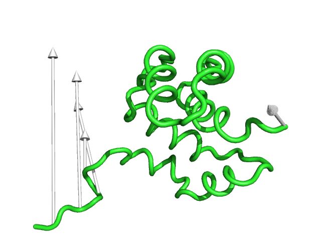
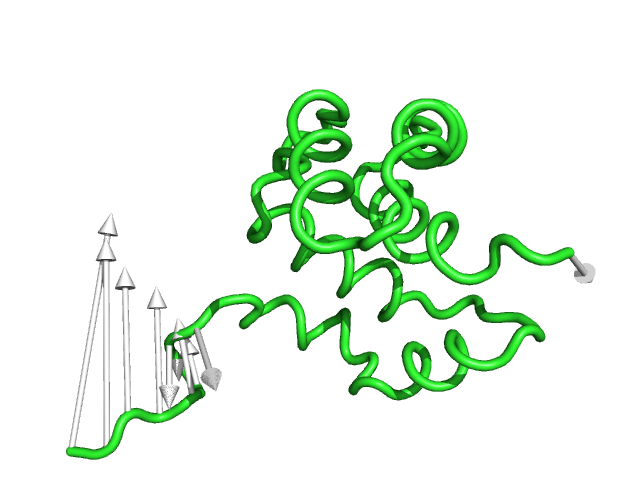
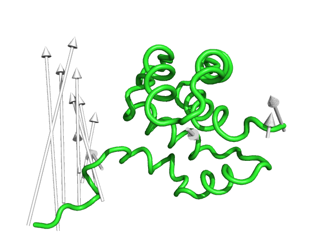
modevectors.py is a PyMol script that was originally written to visualize results obtained from Normal Mode Analysis (NMA) by drawing arrows or vectors from a starting structure to a final structure. However, this script can be used to visualize the direction of motion between two specified states (e.g. targeted MD, comparing open and closed structures, etc). The strength of this script is that the arrows are highly customizable with numerous options to choose from (see script below). It is important to note that the two states MUST be identical except for the X, Y, and Z coordinates. That is, you cannot draw vectors between homologous structures. The default settings sets the background to white and displays the arrows along with the first object frame (in cartoon representation).
Note: Ray tracing these CGO arrows appears to be a memory intensive process so please save a session before ray tracing and use "pymol -qc" where necessary. If anybody can come up with a method to improve this please e-mail me (see address in script).
Update: A new way of drawing the arrows has been implemented for PyMOL v.1.1 and has been updated in this code (which automatically detects the version that you are using). The new method uses the built in cone primitive rather than concentric circles decreasing in size. Thus, the new method is much less memory intensive and is a significant improvement over the old method. Additionally, you may want to turn off ray shadow depending on the scene that you are viewing as shadows can be confusing to others when seen in publications.
USAGE
load the script using the run command
modevectors first_obj_frame, last_obj_frame [,first_state=1 [,last_state=1 [,outname=modevectors \
  [,head=1.0 [,tail=0.3 \[,head_length=1.5 [,headrgb=(1.0,1.0,1.0) [,tailrgb=(1.0,1.0,1.0) [,cutoff=4.0
  [,skip=0 [,cut=0.5 [,atom=CA [,stat=show [,factor=1.0 [,notail=0]]]]]]]]]]]]]]
Please see the script comments for further custom options. Once the script completes, it will generate a new object called "modevectors" (which can be changed through the options).
EXAMPLES
modevectors 1E3M, 1W7A
modevectors 1E3M, 1W7A, outname="arrows"
modevectors 1E3M, 1W7A, atom="P"
Copy/paste the following code to see an example of modevectors. This uses a multistate protein and the arrows are connected between the first and last states.
import modevectors
# fetch the PDBs from pdb.org
fetch 1c3y, finish=1, multiplex=0, async=0
# separate the first and last states of the NMR ensemble to individual objects
split_states 1c3y, 1, 1
split_states 1c3y, 23, 23
hide
# run the modevectors code
modevectors 1c3y_0001, 1c3y_0023
# just setup a nice representation
as cartoon, 1c3y_0001 or 1c3y_0023
show cgo, modevectors
color marine, 1c3y_0001
color purpleblue, 1c3y_0023
The following set of examples will illustrate the power of each optional argument. Each example should be compared to the default figure in the table below.
reinitialize
import modevectors

fetch 1c3y, async=0

split_states 1c3y, 1, 1
split_states 1c3y, 23, 23
hide

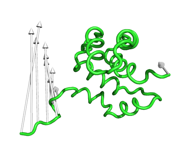
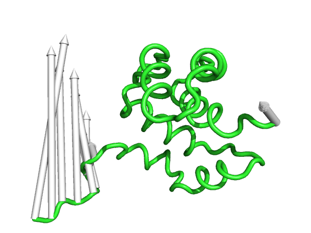
#This is the default setting (Fig.1)
modevectors 1c3y_0001, 1c3y_0023

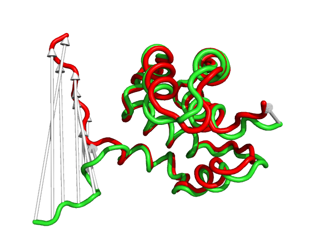
#This is shows that the direction of the arrows is drawn from the 1c3y_0001 towards 1c3y_0023 (Fig.2)
show cartoon, 1c3y_0023
color red, 1c3y_0023

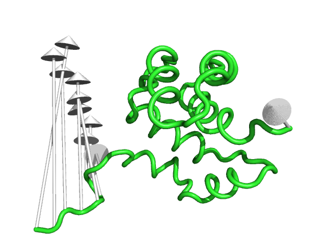
#This controls the base radius of the cone/arrow head in angstroms (Fig.3)
modevectors 1c3y_0001, 1c3y_0023, head=2.5

#This controls the radius of the cylinders/arrow tails in angstroms (Fig.4)
modevectors 1c3y_0001, 1c3y_0023, tail=0.75

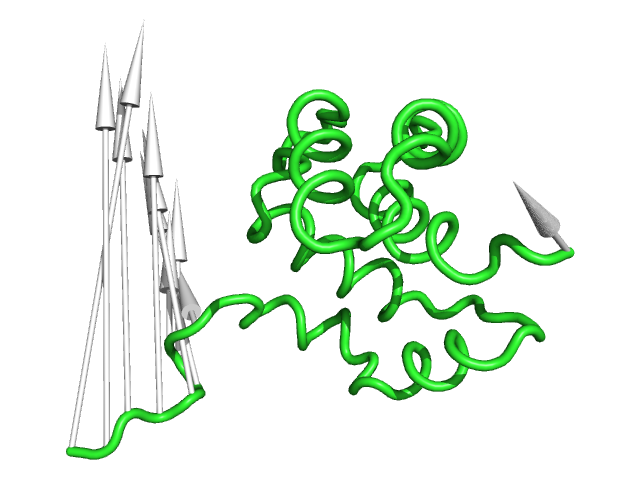
#This controls the length of the cone/arrow head in angstroms (Fig.5)
#Note that this option does NOT increase the vector length but simply changes the tail length
modevectors 1c3y_0001, 1c3y_0023, head_length=3.0

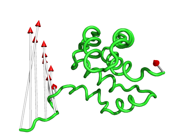
#This controls the colour of the cone/arrow head using RGB values (Fig.6)
modevectors 1c3y_0001, 1c3y_0023, headrgb=(1.0,0.0,0.0)

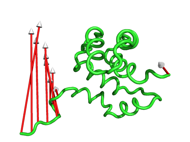
#This controls the colour of the cylinder/arrow tails using RGB values (Fig.7)
modevectors 1c3y_0001, 1c3y_0023, tailrgb=(1.0,0.0,0.0)

#This controls the which vectors to show based on a specific cutoff value in angstroms.  Vector lengths that are less
#than the cutoff value will not be displayed (Fig.8)
modevectors 1c3y_0001, 1c3y_0023, cutoff=30.0

#This controls how many vectors to skip (integer value) and is useful when there are too many vectors showing.
#Skip=1 will show every other arrow (Fig.9)
modevectors 1c3y_0001, 1c3y_0023, skip=1

#This controls how much to cut from each vector (in angstroms).  Note that arrows will point in the opposite directions
#when too much is cutoff (resulting in a negative vector length) (Fig.10) and should be used with caution!
modevectors 1c3y_0001, 1c3y_0023, cut=15.0

#This controls which atom to draw a vector from (Fig.11).  Note that this is case-sensitive and is really only useful
#when atom=CA or when atom=P (for DNA backbones)
modevectors 1c3y_0001, 1c3y_0023, atom=CB

#This controls how much to multiple the length of each vector by (percentage increase/decrease) (Fig.12)
#This example halves the length of each vector (50%)
modevectors 1c3y_0001, 1c3y_0023, factor=0.5

#This hides the statistics which count atoms skipped, atoms counted (number of arrows showing), and number of atoms
#that did not meet the cutoff and are not shown
modevectors 1c3y_0001, 1c3y_0023, stat=hide

#This example shows multiple options being used (Fig.13)
modevectors 1c3y_0001, 1c3y_0023, head=2.0, tail=1.0, head_length=2.0, headrgb=(1.0,0.0,0.0), tailrgb=(0.0,0.0,1.0),
cutoff=0.0,skip=0,cut=0,atom=CA,factor=0.8

#Finally, this example hides all arrow tails and only uses arrow heads via the notail option(No Figure)
modevectors 1c3y_0001, 1c3y_0023, head=2.0, cutoff=0.0,skip=0,cut=0,atom=CA,factor=0.8, notail=1
